
Pandas#
In this chapter we will be discussing the advatages to using the Pandas package to analyze large datasets. While NumPy is a useful package, it can only be used with data of the same datatype. Pandas, however, is a package that helps us manipulate and analyze heterogenous data.
We strongly recommend looking at “10 minutes to pandas” for a broader overview, but here we’ll introduce the main concepts needed for the activities in this textbook.
Before we can use pandas, we need to import it. We can also nickname the modules when we import them. The convention is to import pandas as pd.
# Import packages
import pandas as pd

# Use whos 'magic command' to see available modules
%whos
Variable   Type      Data/Info
------------------------------
pd         module    <module 'pandas' from '/U<...>ages/pandas/__init__.py'>
Create and Manipulate Dataframes#
The two data structures of Pandas are the Series and the DataFrame. A Series is a one-dimensional onject similar to a list. A DataFrame can be thought of as a two-dimensional numpy array or a collection of Series objects. Series and dataframes can contain multiple different data types such as integers, strings, and floats, similar to an Excel spreadsheet. Pandas also supports string lables unlike numpy arrays which only have numeric labels for their rows and columns. For a more in depth explanation, please visit the Introduction to Data Structures section in the Pandas User Guide.
You can create a Pandas dataframe by inputting dictionaries into the Pandas function pd.DataFrame(), by reading files, or through functions built into the Pandas package. The function pd.read_csv() reads a comma- or tab-separated file and returns it as a dataframe.
DataFrame example#
Below we will create a dataframe by reading the file brainarea_vs_genes_exp_w_reannotations.tsv which contains information on gene expression accross multiple brain areas.
About this dataset: This dataset was created by Derek Howard and Abigail Mayes for the purpose of accelerating advances in data mining of open brain transcriptome data for polygenetic brain disorders. The data comes from normalized microarray datasets of gene expression from 6 adult human brains that was released by the Allen Brain Institute and then processed into the dataframe we will see below. For more information on this dataset please visit the HBAsets repository.
# Read in the list of lists as a data frame
file_name = 'brainarea_vs_genes_exp_w_reannotations.tsv'
gene_df = pd.read_csv(file_name, sep='\t')

# '.head()' returns the first 5 rows in the dataframe
gene_df.head()
| gene_symbol | CA1 field | CA2 field | CA3 field | CA4 field | Crus I, lateral hemisphere | Crus I, paravermis | Crus II, lateral hemisphere | Crus II, paravermis | Edinger-Westphal nucleus | ... | temporal pole, inferior aspect | temporal pole, medial aspect | temporal pole, superior aspect | transverse gyri | trochlear nucleus | tuberomammillary nucleus | ventral tegmental area | ventromedial hypothalamic nucleus | vestibular nuclei | zona incerta | |
|---|---|---|---|---|---|---|---|---|---|---|---|---|---|---|---|---|---|---|---|---|---|
| 0 | A1BG | 0.856487 | -1.773695 | -0.678679 | -0.986914 | 0.826986 | 0.948039 | 0.935427 | 1.120774 | -1.018554 | ... | 0.277830 | 0.514923 | 0.733368 | -0.104286 | -0.910245 | 1.039610 | -0.155167 | -0.444398 | -0.901361 | -0.236790 |
| 1 | A1BG-AS1 | 0.257664 | -1.373085 | -0.619923 | -0.636275 | 0.362799 | 0.353296 | 0.422766 | 0.346853 | -0.812015 | ... | 1.074116 | 0.821031 | 1.219272 | 0.901213 | -1.522431 | 0.598719 | -1.709745 | -0.054156 | -1.695843 | -1.155961 |
| 2 | A1CF | -0.089614 | -0.546903 | 0.282914 | -0.528926 | 0.507916 | 0.577696 | 0.647671 | 0.306824 | 0.089958 | ... | -0.030265 | -0.187367 | -0.428358 | -0.465863 | -0.136936 | 1.229487 | -0.110680 | -0.118175 | -0.139776 | 0.123829 |
| 3 | A2M | 0.552415 | -0.635485 | -0.954995 | -0.259745 | -1.687391 | -1.756847 | -1.640242 | -1.733110 | -0.091695 | ... | -0.058505 | 0.207109 | -0.161808 | 0.183630 | 0.948098 | -0.977692 | 0.911896 | -0.499357 | 1.469386 | 0.557998 |
| 4 | A2ML1 | 0.758031 | 1.549857 | 1.262225 | 1.338780 | -0.289888 | -0.407026 | -0.358798 | -0.589988 | 0.944684 | ... | -0.472908 | -0.598317 | -0.247797 | -0.282673 | 1.396365 | 0.945043 | 0.158202 | 0.572771 | 0.073088 | -0.886780 |
5 rows × 233 columns
At the moment, the first column of information above, the index just contains a list of numbers. We can reassign the row labels by using the method set_index(). We can choose any column in our present dataframe to be the row values. Let’s assign the row lables to be the gene_symbol and reassign the dataframe.
row_index = 'gene_symbol'
gene_df = gene_df.set_index(row_index)
gene_df.head()
| CA1 field | CA2 field | CA3 field | CA4 field | Crus I, lateral hemisphere | Crus I, paravermis | Crus II, lateral hemisphere | Crus II, paravermis | Edinger-Westphal nucleus | Heschl's gyrus | ... | temporal pole, inferior aspect | temporal pole, medial aspect | temporal pole, superior aspect | transverse gyri | trochlear nucleus | tuberomammillary nucleus | ventral tegmental area | ventromedial hypothalamic nucleus | vestibular nuclei | zona incerta | |
|---|---|---|---|---|---|---|---|---|---|---|---|---|---|---|---|---|---|---|---|---|---|
| gene_symbol | |||||||||||||||||||||
| A1BG | 0.856487 | -1.773695 | -0.678679 | -0.986914 | 0.826986 | 0.948039 | 0.935427 | 1.120774 | -1.018554 | 0.170282 | ... | 0.277830 | 0.514923 | 0.733368 | -0.104286 | -0.910245 | 1.039610 | -0.155167 | -0.444398 | -0.901361 | -0.236790 |
| A1BG-AS1 | 0.257664 | -1.373085 | -0.619923 | -0.636275 | 0.362799 | 0.353296 | 0.422766 | 0.346853 | -0.812015 | 0.903358 | ... | 1.074116 | 0.821031 | 1.219272 | 0.901213 | -1.522431 | 0.598719 | -1.709745 | -0.054156 | -1.695843 | -1.155961 |
| A1CF | -0.089614 | -0.546903 | 0.282914 | -0.528926 | 0.507916 | 0.577696 | 0.647671 | 0.306824 | 0.089958 | 0.149820 | ... | -0.030265 | -0.187367 | -0.428358 | -0.465863 | -0.136936 | 1.229487 | -0.110680 | -0.118175 | -0.139776 | 0.123829 |
| A2M | 0.552415 | -0.635485 | -0.954995 | -0.259745 | -1.687391 | -1.756847 | -1.640242 | -1.733110 | -0.091695 | 0.003428 | ... | -0.058505 | 0.207109 | -0.161808 | 0.183630 | 0.948098 | -0.977692 | 0.911896 | -0.499357 | 1.469386 | 0.557998 |
| A2ML1 | 0.758031 | 1.549857 | 1.262225 | 1.338780 | -0.289888 | -0.407026 | -0.358798 | -0.589988 | 0.944684 | -0.466327 | ... | -0.472908 | -0.598317 | -0.247797 | -0.282673 | 1.396365 | 0.945043 | 0.158202 | 0.572771 | 0.073088 | -0.886780 |
5 rows × 232 columns
It would help to know what information is in our dataset. In other words, what is across the columns at the top? We can get a list by accessing the columns attribute.
# Access the columns of our dataframe
gene_df_columns = gene_df.columns
gene_df_columns
Index(['CA1 field', 'CA2 field', 'CA3 field', 'CA4 field',
       'Crus I, lateral hemisphere', 'Crus I, paravermis',
       'Crus II, lateral hemisphere', 'Crus II, paravermis',
       'Edinger-Westphal nucleus', 'Heschl's gyrus',
       ...
       'temporal pole, inferior aspect', 'temporal pole, medial aspect',
       'temporal pole, superior aspect', 'transverse gyri',
       'trochlear nucleus', 'tuberomammillary nucleus',
       'ventral tegmental area', 'ventromedial hypothalamic nucleus',
       'vestibular nuclei', 'zona incerta'],
      dtype='object', length=232)
Indexing Dataframes#
Indexing in Pandas works slightly different than in NumPy. Similar to a dictionary, we can index dataframes by their names.
The syntax for indexing single locations in a dataframe is dataframe.loc[row_label,column_label]. To index an individual column, we use the shorthand syntax dataframe.[column_label]. To index an individual row, we use the syntax dataframe.loc[row_label]. To index by index #, we use the syntax dataframe.iloc[index_number]. Below are some examples on how to access rows, columns, and single values in our dataframe. For more information on indexing dataframes, visit the “Indexing and selecting data” section in the Pandas User Guide.
# Select a single column
column = 'CA1 field'
print('Gene expression values in CA1 field:')
gene_df[column]
Gene expression values in CA1 field:
gene_symbol
A1BG        0.856487
A1BG-AS1    0.257664
A1CF       -0.089614
A2M         0.552415
A2ML1       0.758031
              ...
ZYG11A     -0.496398
ZYG11B     -0.856866
ZYX        -1.941816
ZZEF1      -0.015748
ZZZ3       -0.924901
Name: CA1 field, Length: 20869, dtype: float64
# Select a single row
row = 'A1BG'
print('Gene expression of ', row, ' across brain regions:')
gene_df.loc[row]
Gene expression of A1BG across brain regions:
CA1 field                            0.856487
CA2 field                           -1.773695
CA3 field                           -0.678679
CA4 field                           -0.986914
Crus I, lateral hemisphere           0.826986
                                       ...
tuberomammillary nucleus             1.039610
ventral tegmental area              -0.155167
ventromedial hypothalamic nucleus   -0.444398
vestibular nuclei                   -0.901361
zona incerta                        -0.236790
Name: A1BG, Length: 232, dtype: float64
# Select an individual value
print('Gene expression of A1BG in CA1 field:')
gene_df.loc[row, column]
Gene expression of A1BG in CA1 field:
0.8564873784944677
To select multiple different columns, you can use a list of all your columns of interest as so:
# Select multiple columns
print('Gene expression values in multiple regions :')
columns = ['CA1 field', 'CA3 field', 'Crus I, lateral hemisphere']
gene_df[columns]
Gene expression values in multiple regions :
| CA1 field | CA3 field | Crus I, lateral hemisphere | |
|---|---|---|---|
| gene_symbol | |||
| A1BG | 0.856487 | -0.678679 | 0.826986 |
| A1BG-AS1 | 0.257664 | -0.619923 | 0.362799 |
| A1CF | -0.089614 | 0.282914 | 0.507916 |
| A2M | 0.552415 | -0.954995 | -1.687391 |
| A2ML1 | 0.758031 | 1.262225 | -0.289888 |
| ... | ... | ... | ... |
| ZYG11A | -0.496398 | 0.325555 | 0.158885 |
| ZYG11B | -0.856866 | 0.701878 | 0.337138 |
| ZYX | -1.941816 | -0.681255 | 0.872683 |
| ZZEF1 | -0.015748 | 0.743609 | 1.108376 |
| ZZZ3 | -0.924901 | 0.108320 | -1.591413 |
20869 rows × 3 columns
Subsetting#
Like NumPy arrays, we can subset our original dataframe to only include data that meets our criteria. Our dataframe has data on multiple different brain areas with many gene expression values. You can filter this dataframe using the following syntax:
new_df = original_df[original_df['Column of Interest'] == 'Desired Value']
In plain english, what this is saying is: save a dataframe from the original dataframe, where the original dataframe values in my Column of Interest are equal to my Desired Value. For more information on subsetting, visit the “How do I select a subset of a DataFrame” section in the Pandas documentation.
Below we will demonstrate how to execute this by taking a look at the CA1 field column in gene_df. We will create a dataframe from gene_df that only contains genes that showed a certain level of gene expression.
# Create a dataframe with only genes that have an expression
# value greater than 1.7 in 'CA1 field'
desired_column = 'CA1 field'
desired_value = 1.7
new_gene_df = gene_df[gene_df[desired_column] > desired_value]
new_gene_df.head()
| CA1 field | CA2 field | CA3 field | CA4 field | Crus I, lateral hemisphere | Crus I, paravermis | Crus II, lateral hemisphere | Crus II, paravermis | Edinger-Westphal nucleus | Heschl's gyrus | ... | temporal pole, inferior aspect | temporal pole, medial aspect | temporal pole, superior aspect | transverse gyri | trochlear nucleus | tuberomammillary nucleus | ventral tegmental area | ventromedial hypothalamic nucleus | vestibular nuclei | zona incerta | |
|---|---|---|---|---|---|---|---|---|---|---|---|---|---|---|---|---|---|---|---|---|---|
| gene_symbol | |||||||||||||||||||||
| ABCC12 | 2.089999 | 0.684837 | 0.097313 | -0.051411 | -1.078900 | -0.912071 | -1.131497 | -0.799075 | -0.009423 | 0.889132 | ... | 1.289340 | 0.885886 | 1.271053 | 0.650801 | -0.083413 | -0.793237 | -0.499512 | -0.762330 | -0.902496 | -0.904421 |
| ABHD17C | 1.716973 | 0.601041 | 1.132500 | 1.354679 | -0.923195 | -0.887576 | -1.122027 | -0.926876 | 0.339678 | 0.208174 | ... | 0.530983 | 0.809101 | 0.763170 | -0.093598 | -0.313468 | -0.164013 | -0.537971 | 1.169105 | -0.663245 | -0.377181 |
| ABI1 | 2.051762 | 2.571777 | 2.472188 | 2.261170 | 0.366138 | 0.507783 | 0.449606 | 0.498424 | -1.365242 | 0.472104 | ... | 0.868471 | 1.197022 | 0.914783 | 0.473846 | -2.230209 | -0.330684 | -1.153189 | -0.073650 | -1.681602 | -1.049258 |
| ACTB | 2.489711 | 2.806688 | 2.461655 | 2.340131 | -1.296731 | -1.334696 | -1.158460 | -1.461027 | 0.088209 | 0.027236 | ... | -0.370215 | -0.946920 | -0.197363 | -0.094468 | 0.926183 | -0.034337 | 0.803164 | -0.389238 | 0.596916 | 0.110921 |
| ACTR2 | 2.655049 | 2.384445 | 1.728348 | 1.413585 | -1.377474 | -1.207922 | -1.496018 | -1.359462 | 0.632764 | 0.259402 | ... | 0.215683 | 0.142880 | 0.080649 | 0.312218 | 1.793563 | -0.028263 | -0.189930 | -0.389064 | -0.484580 | -1.478232 |
5 rows × 232 columns
DataFrame Methods#
Pandas has many useful methods that you can use on your data, including describe, mean, and more. To learn more about all the different methods that can be used to manipulate and analyze dataframes, please visit the Pandas User Guide . We will demonstrate some of these methods below.
The describe method returns descriptive statistics of all the columns in our dataframe.
gene_df.describe()
| CA1 field | CA2 field | CA3 field | CA4 field | Crus I, lateral hemisphere | Crus I, paravermis | Crus II, lateral hemisphere | Crus II, paravermis | Edinger-Westphal nucleus | Heschl's gyrus | ... | temporal pole, inferior aspect | temporal pole, medial aspect | temporal pole, superior aspect | transverse gyri | trochlear nucleus | tuberomammillary nucleus | ventral tegmental area | ventromedial hypothalamic nucleus | vestibular nuclei | zona incerta | |
|---|---|---|---|---|---|---|---|---|---|---|---|---|---|---|---|---|---|---|---|---|---|
| count | 20869.000000 | 20869.000000 | 20869.000000 | 20869.000000 | 20869.000000 | 20869.000000 | 20869.000000 | 20869.000000 | 20869.000000 | 20869.000000 | ... | 20869.000000 | 20869.000000 | 20869.000000 | 20869.000000 | 20869.000000 | 20869.000000 | 20869.000000 | 20869.000000 | 20869.000000 | 20869.000000 |
| mean | 0.003664 | 0.017002 | 0.015315 | -0.016633 | 0.093686 | 0.088810 | 0.096118 | 0.087608 | 0.047124 | -0.042517 | ... | -0.056050 | -0.051731 | -0.049905 | -0.039528 | 0.059726 | 0.014856 | 0.009535 | -0.002853 | -0.002527 | 0.013018 |
| std | 0.924456 | 1.129368 | 1.078987 | 0.897192 | 1.146146 | 1.118501 | 1.172986 | 1.136823 | 0.973224 | 0.500526 | ... | 0.567950 | 0.651098 | 0.636729 | 0.494012 | 1.158916 | 0.897387 | 0.686320 | 0.830602 | 0.723977 | 0.725770 |
| min | -4.076424 | -5.923691 | -5.994731 | -3.971984 | -2.739924 | -2.662897 | -2.908676 | -2.864308 | -3.671242 | -1.666268 | ... | -1.840486 | -2.433961 | -2.412614 | -1.655962 | -6.330275 | -3.141490 | -1.977225 | -3.541112 | -2.369304 | -2.348784 |
| 25% | -0.570475 | -0.644093 | -0.631248 | -0.573605 | -0.802651 | -0.778933 | -0.824404 | -0.794683 | -0.651691 | -0.414882 | ... | -0.472481 | -0.517562 | -0.529458 | -0.404416 | -0.751329 | -0.602619 | -0.497988 | -0.542164 | -0.532177 | -0.493921 |
| 50% | -0.025821 | 0.011189 | 0.006140 | -0.044566 | 0.100558 | 0.098665 | 0.109358 | 0.096585 | 0.022760 | -0.057495 | ... | -0.091029 | -0.083971 | -0.089572 | -0.051758 | 0.037410 | -0.030474 | -0.023799 | -0.023471 | -0.045003 | -0.031623 |
| 75% | 0.561571 | 0.706946 | 0.706398 | 0.547903 | 0.985159 | 0.951919 | 1.007791 | 0.960813 | 0.736614 | 0.312739 | ... | 0.352796 | 0.412321 | 0.403382 | 0.310551 | 0.844723 | 0.587382 | 0.503613 | 0.508410 | 0.501191 | 0.492262 |
| max | 7.062717 | 7.387742 | 6.413603 | 7.178692 | 2.679149 | 2.717237 | 2.963899 | 2.857205 | 7.552440 | 2.234669 | ... | 2.199291 | 2.631498 | 3.065735 | 2.238555 | 6.892682 | 5.968364 | 7.267837 | 6.650673 | 2.723777 | 2.845665 |
8 rows × 232 columns
The mean and std method return the mean and standard deviation of each column in the dataframe, respectfully.
gene_df.mean()
CA1 field                            0.003664
CA2 field                            0.017002
CA3 field                            0.015315
CA4 field                           -0.016633
Crus I, lateral hemisphere           0.093686
                                       ...
tuberomammillary nucleus             0.014856
ventral tegmental area               0.009535
ventromedial hypothalamic nucleus   -0.002853
vestibular nuclei                   -0.002527
zona incerta                         0.013018
Length: 232, dtype: float64
gene_df.std()
CA1 field                            0.924456
CA2 field                            1.129368
CA3 field                            1.078987
CA4 field                            0.897192
Crus I, lateral hemisphere           1.146146
                                       ...
tuberomammillary nucleus             0.897387
ventral tegmental area               0.686320
ventromedial hypothalamic nucleus    0.830602
vestibular nuclei                    0.723977
zona incerta                         0.725770
Length: 232, dtype: float64
Let’s say we have two different dataframes and we would like to combine the two into one single dataframe. We can use either the merge or join Pandas methods in order to pull all of this data into one dataframe.
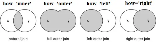
There are different types of joins/merges you can do in Pandas, illustrated above. Here, we want to do an inner merge, where we’re only keeping entries with indices that are in both dataframes. We could do this merge based on columns, alternatively.
Inner is the default kind of join, so we do not need to specify it. And by default, join will use the ‘left’ dataframe, in other words, the dataframe that is executing the join method.
If you need more information, look at the join and merge documentation: you can use either of these to unite your dataframes, though join will be simpler!
Below is an example of how to join two separate dataframe into one, unified dataframe. We start with one dataframe with only entries from the temporal pole and another dataframe with only entries from the CA fields of the hippocampus. We can then join the two dataframes together using the syntax unified_df = df_1.join(df_2)
# Dataframe w/ only Temporal Pole entries
temporal_pole_df = gene_df[['temporal pole, inferior aspect',
                            'temporal pole, medial aspect',
                            'temporal pole, superior aspect']]
temporal_pole_df.head()
| temporal pole, inferior aspect | temporal pole, medial aspect | temporal pole, superior aspect | |
|---|---|---|---|
| gene_symbol | |||
| A1BG | 0.277830 | 0.514923 | 0.733368 |
| A1BG-AS1 | 1.074116 | 0.821031 | 1.219272 |
| A1CF | -0.030265 | -0.187367 | -0.428358 |
| A2M | -0.058505 | 0.207109 | -0.161808 |
| A2ML1 | -0.472908 | -0.598317 | -0.247797 |
# Dataframe w/ only CA field entries
CA_field_df = gene_df[['CA1 field',
                       'CA2 field',
                       'CA3 field',
                       'CA4 field']]
CA_field_df.head()
| CA1 field | CA2 field | CA3 field | CA4 field | |
|---|---|---|---|---|
| gene_symbol | ||||
| A1BG | 0.856487 | -1.773695 | -0.678679 | -0.986914 |
| A1BG-AS1 | 0.257664 | -1.373085 | -0.619923 | -0.636275 |
| A1CF | -0.089614 | -0.546903 | 0.282914 | -0.528926 |
| A2M | 0.552415 | -0.635485 | -0.954995 | -0.259745 |
| A2ML1 | 0.758031 | 1.549857 | 1.262225 | 1.338780 |
#Join the two dataframes
df_1 = temporal_pole_df
df_2 = CA_field_df

unified_df = df_1.join(df_2)
unified_df.head()
| temporal pole, inferior aspect | temporal pole, medial aspect | temporal pole, superior aspect | CA1 field | CA2 field | CA3 field | CA4 field | |
|---|---|---|---|---|---|---|---|
| gene_symbol | |||||||
| A1BG | 0.277830 | 0.514923 | 0.733368 | 0.856487 | -1.773695 | -0.678679 | -0.986914 |
| A1BG-AS1 | 1.074116 | 0.821031 | 1.219272 | 0.257664 | -1.373085 | -0.619923 | -0.636275 |
| A1CF | -0.030265 | -0.187367 | -0.428358 | -0.089614 | -0.546903 | 0.282914 | -0.528926 |
| A2M | -0.058505 | 0.207109 | -0.161808 | 0.552415 | -0.635485 | -0.954995 | -0.259745 |
| A2ML1 | -0.472908 | -0.598317 | -0.247797 | 0.758031 | 1.549857 | 1.262225 | 1.338780 |
Those are the basics of working with Pandas dataframes! Circle back to this page or the resources linked within if you ever need a refresher. Next, we’ll talk about the power of SciPy for scientific analysis in Python.
Additional resources#
See the Python Data Science Handbook for a more in depth exploration of Pandas, and of course, the Pandas documentation.