
Spike Sorting#
When you record extracellular electrophysiology data, one of the first data processing steps is figuring out which action potentials (or “spikes”) came from which neurons. The process of doing this is called spike sorting.
Below, we’ll work with this dataset from Lisa Giocomo’s lab at Stanford to demonstrate the simplest form of spike sorting: thresholding, followed by feature extraction.
Note #1: The code below requires a different dataset than the one we interacted with in the last chapter. Because this dataset contains all of the raw recording data, it is much, much bigger. As a result, the best way to work with it is by streaming it from DANDI, which works best on the Dandihub. If you’re running locally, ensure you have completed the setup steps in Using this Book, particularly the streaming configuration.
Note #2: Some of the cells below may take a minute to run, depending on the speed of your internet connection.
Step 1. Inspect the Data#
First, we need to find the correct URL for the dataset on the NWB’s Amazon S3 storage system. There is a tool to do so within the dandiapi, which we’ll use below to get the URL for one session within the dataset.
from dandi.dandiapi import DandiAPIClient

dandiset_id = '000053' # giocomo data
filepath = 'sub-npI5/sub-npI5_ses-20190414_behavior+ecephys.nwb'

with DandiAPIClient() as client:
    asset = client.get_dandiset(dandiset_id, 'draft').get_asset_by_path(filepath)
    s3_path = asset.get_content_url(follow_redirects=1, strip_query=True)

print(s3_path)
https://dandiarchive.s3.amazonaws.com/blobs/d6d/882/d6d88284-983a-42a7-91e8-48e9f59c2881
Now that we have this path, we can stream the data using remfile. Below, we’ll print some useful information about this experiment. We will also access a dataset we haven’t interacted with yet: ElectricalSeries. As the name suggests, this group contains raw electrophysiology data – exactly what we need to sort! We will assign a portion of this to an object called ephys_data.
Note: The cell below will take about a minute to run, depending on the speed of your internet connection.
from pynwb import NWBHDF5IO
import h5py
import remfile

# Stream the file using remfile
rem_file = remfile.File(s3_path)

with h5py.File(rem_file, "r") as h5py_file:
    with NWBHDF5IO(file=h5py_file, load_namespaces=True) as io:
        nwbfile = io.read()
        print(nwbfile.acquisition['ElectricalSeries'].data.shape)
        sampling_freq = nwbfile.acquisition['ElectricalSeries'].rate # get the sampling frequency in Hz
        ephys_data = (nwbfile.acquisition['ElectricalSeries'].data[:3000000, 99])*nwbfile.acquisition['ElectricalSeries'].conversion
(235949418, 384)
Before we dive into spike sorting, let’s take a look at the data. Below, we’ll import a couple additional packages, generate a list of timestamps, and plot it.
Need a reminder on how some of the packages or functions below work? Look through the NumPy and Matplotlib review pages.
# import necessary packages
import numpy as np
import matplotlib.pyplot as plt

# generate a vector of timestamps
timestamps = np.arange(0, len(ephys_data)) * (1.0 / sampling_freq)

fig,ax = plt.subplots(1,1,figsize=(15,3))
plt.plot(timestamps,ephys_data)
plt.ylabel('Voltage (V)')
plt.xlabel('Seconds (s)')
#plt.xlim(1.053,1.055)
plt.show()
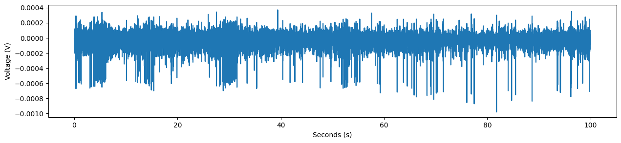
In the data above, there are clear places where the data “spikes”. These are extracellularly recorded action potentials!
plt.xlim() line to change the limits on the x-axis and find a single action potential.Step 2. Spike Detection#
One of the most straightforward ways to spike sort is to simply detect these using a threshold. Whenever the signal passes this threshold, we’ll clip that out. We could determine a reasonable threshold by eye, but we’ll do this mathematically instead, using the standard deviation of the signal. When the signal is five times the standard deviation, that’s enough signal to noise that it’s likely to be an action potential. We’ll calculate that below.
noise_std = np.std(ephys_data)
recommended_threshold = -5 * noise_std
print('Noise Estimate by Standard Deviation: ', noise_std)
print('Recommended Spike Threshold         : ', recommended_threshold)
Noise Estimate by Standard Deviation:  3.0522641151468644e-05
Recommended Spike Threshold         :  -0.00015261320575734322
Our spike detector needs to take into account that a spike typically comprises multiple samples, so we can’t simply take each sample that exceeds the threshold as an individual spike detection. Instead, we’ll define a dead time: whenever we detect a spike, the next few samples within the dead time won’t trigger a spike detection by themselves.
In order to generate a more precise idea of where each spike is we will also search for the minimum in each spike by lookiing through the signal for a short period of time after the threshold crossing. The time of this minimum will be the timestamp for each spike.
Below, we’ll define three helper functions to accomplish this detection strategy:
def detect_threshold_crossings(signal, fs, threshold, dead_time):
    """
    Detect threshold crossings in a signal with dead time.

    The signal transitions from above to below the threshold for a
    detection and the last detection has to be more than dead_time
    apart from the current one.

    :param signal: The signal as a 1-dimensional numpy array
    :param fs: The sampling frequency in Hz
    :param threshold: The threshold for the signal
    :param dead_time: The dead time in seconds.
    """
    dead_time_idx = dead_time * fs
    threshold_crossings = np.diff(
        (signal <= threshold).astype(int) > 0
    ).nonzero()[0]
    distance_sufficient = np.insert(
        np.diff(threshold_crossings) >= dead_time_idx, 0, True
    )
    while not np.all(distance_sufficient):
        # Repeatedly remove threshold crossings that violate dead_time
        threshold_crossings = threshold_crossings[distance_sufficient]
        distance_sufficient = np.insert(
            np.diff(threshold_crossings) >= dead_time_idx, 0, True
        )
    return threshold_crossings


def get_next_minimum(signal, index, max_samples_to_search):
    """
    Return the index of the next minimum in the signal after an index.

    :param signal: The signal as a 1-dimensional numpy array
    :param index: The scalar index
    :param max_samples_to_search: Number of samples to search for minimum
    """
    search_end_idx = min(index + max_samples_to_search, signal.shape[0])
    min_idx = np.argmin(signal[index:search_end_idx])
    return index + min_idx


def align_to_minimum(signal, fs, threshold_crossings, search_range):
    """
    Return the index of the next negative spike peak for all crossings.

    :param signal: The signal as a 1-dimensional numpy array
    :param fs: The sampling frequency in Hz
    :param threshold_crossings: Array of indices where signal crossed
    :param search_range: Maximum duration in seconds to search
    """
    search_end = int(search_range*fs)
    aligned_spikes = [
        get_next_minimum(signal, t, search_end)
        for t in threshold_crossings
    ]
    return np.array(aligned_spikes)
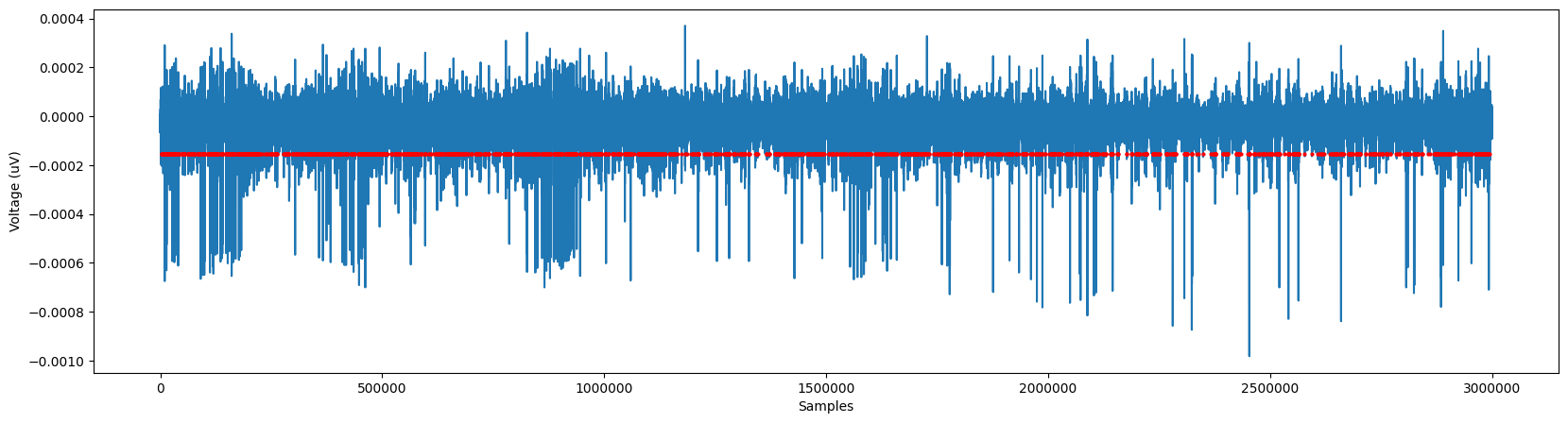
Now, we can use those functions to detect threshold crossings. We’ll then plot our original signal with the detected spikes marked.
crossings = detect_threshold_crossings(ephys_data, sampling_freq, recommended_threshold, 0.003) # dead time of 3 ms
spks = align_to_minimum(ephys_data, sampling_freq, crossings, 0.002) # search range 2 ms

fig,ax = plt.subplots(1,1,figsize=(20,5))
plt.plot(ephys_data)
plt.xlabel('Samples')
plt.ylabel('Voltage (uV)')
plt.plot(spks,[recommended_threshold]*spks.shape[0], 'ro', ms=2)
ax.ticklabel_format(useOffset=False, style='plain')
#plt.xlim([0,len(ephys_data)])
plt.show()
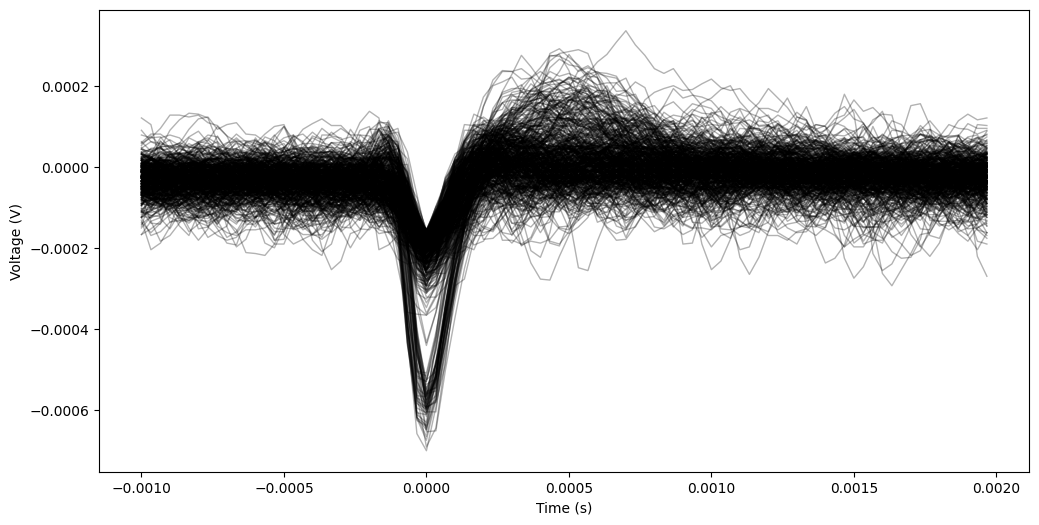
Finally, we can cut out the waveforms from these detected spikes so that we can look at their shape. To do so, we will cut out a portion of the signal around each spike. Spikes too close to the start or end of the signal that a full cutout is not possible are ignored.
The location and shape of a waveform is one of the main pieces of evidence to show that the waveform was recorded from a cell. This will help us determine whether or not there is just one or more neurons recorded on this channel.
Below, we will define two helper functions: one to extract the waveforms, and one to plot them.
def extract_waveforms(signal, fs, spikes_idx, pre, post):
    """
    Extract spike waveforms as signal cutouts around each spike index.

    :param signal: The signal as a 1-dimensional numpy array
    :param fs: The sampling frequency in Hz
    :param spikes_idx: The sample index of all spikes as a 1-dim array
    :param pre: The duration of the cutout before the spike in seconds
    :param post: The duration of the cutout after the spike in seconds
    """
    cutouts = []
    pre_idx = int(pre * fs)
    post_idx = int(post * fs)
    for index in spikes_idx:
        if index-pre_idx >= 0 and index+post_idx <= signal.shape[0]:
            cutout = signal[(index-pre_idx):(index+post_idx)]
            cutouts.append(cutout)
    return np.stack(cutouts)


def plot_waveforms(cutouts, fs, pre, post, n=100):
    """
    Plot an overlay of spike cutouts.

    :param cutouts: A spikes x samples array of cutouts
    :param fs: The sampling frequency in Hz
    :param pre: The duration of the cutout before the spike in seconds
    :param post: The duration of the cutout after the spike in seconds
    :param n: Number of cutouts to plot, or None to plot all. Default: 100
    """
    if n is None:
        n = cutouts.shape[0]
    n = min(n, cutouts.shape[0])
    time_in_us = np.arange(-pre, post, 1/fs)
    plt.figure(figsize=(12,6))

    for i in range(n):
        plt.plot(
            time_in_us, cutouts[i,],
            color='k', linewidth=1, alpha=0.3
        )
        plt.xlabel('Time (s)')
        plt.ylabel('Voltage (V)')

    plt.show()
Now, let’s extract & plot the waveforms.
try:
    pre = 0.001 # 1 ms
    post= 0.002 # 2 ms
    waveforms = extract_waveforms(ephys_data, sampling_freq, spks, pre, post)
    plot_waveforms(waveforms, sampling_freq, pre, post, n=500)
    min_voltage = np.amin(waveforms, axis=1)
    max_voltage = np.amax(waveforms, axis=1)

except ValueError:
    print('No data loaded.')
    min_voltage, max_voltage = 0,0
Step 3. Feature Extraction#
Indeed, it looks like there might be two – one that is very high amplitude, and another that is lower amplitude. We can use feature extraction to investigate our waveforms. Below, we’ll plot the minimum and maximum voltages in the recorded waveforms to see if there are distinct clusters of waveforms.
plt.figure(figsize=(8,8))
plt.plot(min_voltage, max_voltage,'.')
plt.xlabel('Minimum Voltage (V)')
plt.ylabel('Maximum Voltage (V)')
plt.title('Min/Max Spike Voltages')

plt.show()
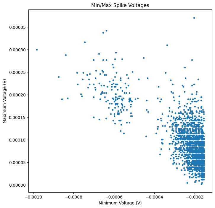
Looking at the scatterplot above, would you say there is more than one cluster of waveforms?
For these two units, separating by minimum & maximum voltage actually works fairly well! However, many action potentials have shapes that cannot be easily summarized by one feature such as the minimum voltage. For this, a more general feature extraction method such as principal component analysis (PCA) is typically used.
Notebook summary#
In this notebook, we’ve looked closely at just 100 seconds of one channel in a 384-channel recording. You can imagine how long spike sorting would take if we needed to do this for all of the data. Thankfully, there are more automated spike sorting tools which enable researchers to automatically sort their data, with just a little bit of sorting by hand (e.g., Kilosort.
In the next notebook, we’ll work with data that has already been sorted for us. The resulting dataset has spike times for each sorted neuron (or “unit”) – the moments in the experiment where a spike happened. This is the most common format for data sharing of extracellularly recorded data, since it’s much more concise, and the hard work of spike sorting has already happened.
Notes & resources#
This notebook borrows inspiration and code from this tutorial which is protected under a copyright: Copyright (c) 2018, Multi Channel Systems MCS GmbH All rights reserved.